A Glimpse at RAI scores in East Asia

RAI

Data Visualization

Multi-Level Systems

East Asia

In this post, we take a look at RAI scores across East Asia

Author

Lucas Couto

Published

July 24, 2024

This Month’s Visualisation

Hello everyone!

In this month’s post, we take a look at the Regional Authority Index (RAI) in East Asia! But why so? In the last months, I’ve been reading some scholarship about the countries in the region, such as a recent piece on how academic research can have a meaningful impact on the perception of election integrity, with evidence from South Korea, and experimental evidence from Japan warning how gender bias is present even in the details, manifested through the preference for lower-pitched candidates. I’ve also read a pretty interesting comparative work on coalition governments in Asian-Pacific democracies. I’m sure there’s much more I still haven’t put my hands on, but that was enough to spark my interest in the region!

Though all of this certainly has led me to explore East Asia now, there’s also a personal reason for it. Well, the fact is that I’ve made a few visualisations about Africa before, some about Europe, a lot about the American continent,¹ and recently explored Oceania through New Zealand’s partisan politics. It’s finally time to finish covering all the continents (apart from Antarctica duhh) with Asia now!

Regional Authority Index (RAI)

So, what is the Regional Authority Index (RAI)? In a few words, the RAI is a measure that captures to what extent power (or authority) is shared and exercised by regional governments in each country. The centrepiece of the RAI is dividing the concept of authority into two dimensions: self-rule and shared rule. The former tells us the degree to which each regional government can exercise power within its bounds, whereas the latter tells us whether and to what extent regional governments have a say on national matters.

In summary, RAI provides us with the tools to examine power-sharing in multi-level systems. Below, my main concern is to inspect whether East Asian countries concentrate power on the national government or whether it is reasonably shared among subnational entities. Before proceeding, it is worth pointing out that each dimension (self-rule and shared rule) is formed by five constituent parts, and you can read more about each in Hooghe et al. (2010), Hooghe et al. (2016), and Shair-Rosenfield et al. (2021).

A Choropleth Map

The visualisation below is a map. More accurately, a bichoropleth map! Choropleth maps are nothing more than maps that use colours to enumerate territories along a single category (for ex., # of football teams per state) or to represent different categories. As a consequence, a bichoropleth map serves to identify how territorial units fare along two dimensions. This is perfect to use along with RAI scores, which precisely rely on two super-dimensions.

Several tutorials on the internet provide the steps to make choropleth maps (e.g., here). I’ll rely on a great visualisation made by Moriah Taylor two years ago. By the way, it amazes me how time passes, and I still refer back to Taylor’s “dated” visualisation to use it as inspiration/basis. She is great!

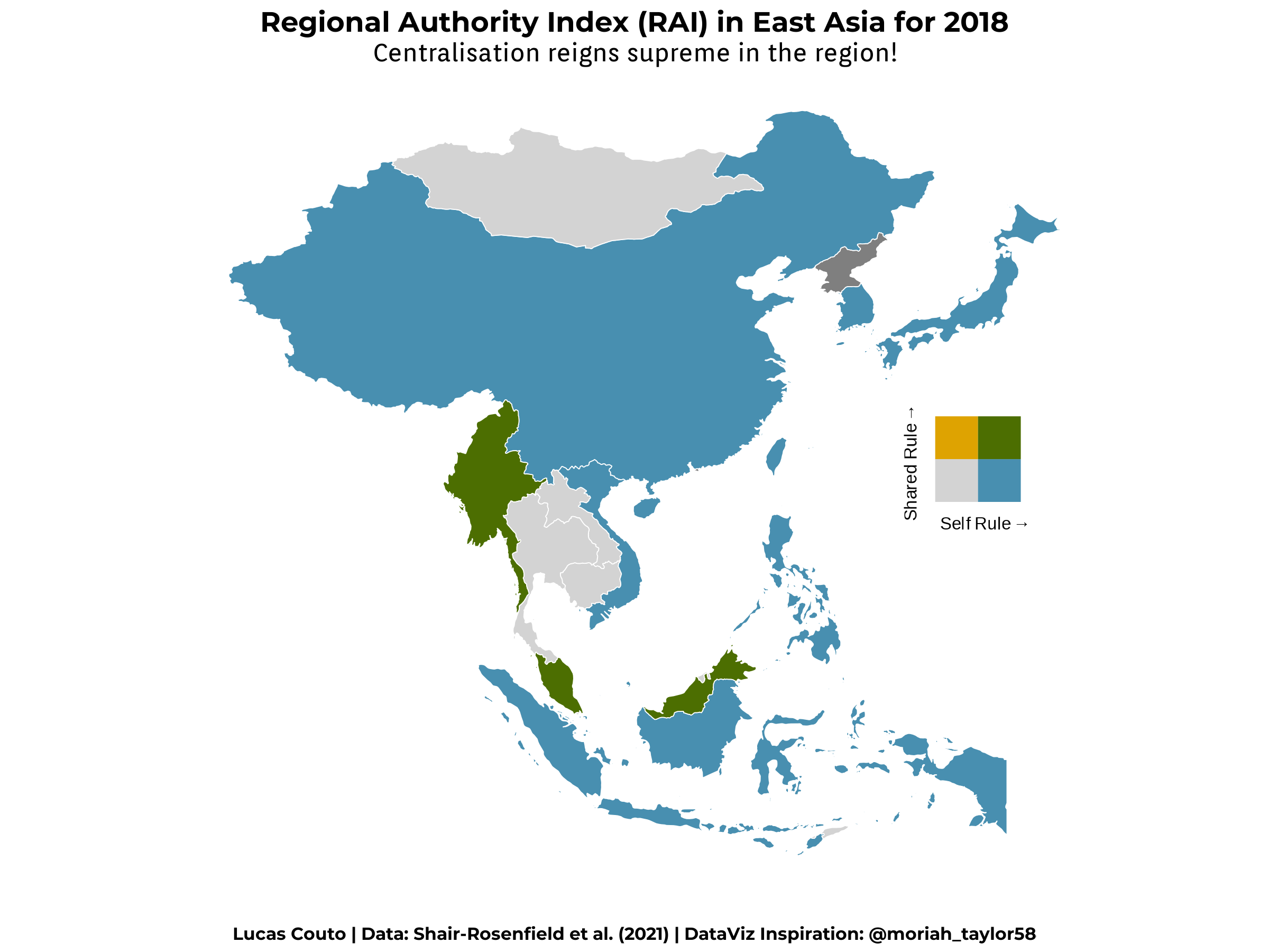
RAI Scores in East Asia

The figure above generates interesting insights, but before let’s see how to interpret the map first. The most important aspect is that the legend (the 2x2 square) serves as our compass to navigate the map. As can be seen, Self-Rule is on the x-axis, and Shared Rule is on the y-axis. The grey square indicates countries where regional governments have neither significant scores on self-rule, nor on shared rule. In other words, countries whose national governments stack the cards all in their favour. Next, the steel blue represents countries where regional governments have enough authority to exert influence within their borders, but not enough to have a say on national matters. Contrariwise, the orange, corn-ish colour indicates the opposite: regional governments with influence on national policies, but not so much on their own territory. Lastly, the green indicates countries where regional governments are important in both dimensions.

Overall, regional governments have a limited scope of influence in the region. First, the figure shows us several countries in grey (Brunei, Cambodia, East Timor, Laos, Mongolia, Singapore, and Thailand). Although other countries grant regional governments substantial authority in what concerns the territories’ own governance, they nonetheless lack the power to influence national politics more broadly (e.g., China, Indonesia, Japan, South Korea, the Philippines, Taiwan, and Vietnam). The opposite is not even found in the chart. To conclude, only two countries sufficiently scores on the two dimensions to grant considerable autonomy to regional governments: Myanmar and Malaysia. Even still, both Myanmar (self-rule: 7.99 and shared rule: 4.89) and Malaysia (self-rule: 13.99 and shared rule: 7.48) are very distant from the scores of some Western democracies, such as Belgium (self-rule: 22.39 and shared rule: 11.47) and Germany (self-rule: 25.67 and shared rule: 12).

By the way, we don’t have values for North Korea and, for this reason, the country is in dark grey😔

That’s it for this month. See you shortly with a thematic plot for August!!

Code

Show the code

##before you proceed, you should download the RAI-country dataset from https://garymarks.web.unc.edu/data/regional-authority-2/

#Load packages
library(biscale)
library(classInt)
library(cowplot) 
library(ggtext)
library(ragg)
library(readxl)
library(rmapshaper)
library(rnaturalearth)
library(rnaturalearthdata)
library(showtext)
library(sf)
library(tidyverse)

#map data
world <- ne_countries(scale = "medium", 
                      returnclass = "sf")

east_asia <- world %>%
             filter(region_wb == "East Asia & Pacific") %>%
             filter(region_un == "Asia")

country_list <- east_asia %>%
                select(sovereignt) %>%
                st_set_geometry(NULL) %>%
                unique() %>%
                pull()

#load RAI data
rai <- read_xlsx("RAI_country-april-2021.xlsx")

uncover_median <- rai %>%
                  select(country_name, n_selfrule, n_sharedrule) %>%
                  unique() %>%
                  mutate(median_selfrule = median(n_selfrule),
                         median_sharedrule = median(n_sharedrule)) %>%
                  filter(country_name %in% country_list) %>%
                  select(-n_selfrule, -n_sharedrule) %>%
                  unique()
       
rai_2 <- rai %>%
         filter(year == 2018) %>%
         filter(country_name %in% country_list) %>%
         left_join(uncover_median) %>%
         select("name" = country_name, n_selfrule, n_sharedrule, median_selfrule, median_sharedrule) %>%
         mutate(name = case_when(name == "South Korea" ~ "Korea",
                                 name == "Laos" ~ "Lao PDR",
                                 name == "East Timor" ~ "Timor-Leste",
                                 T ~ as.character(name)))

#Maps
east_asia_points <- st_centroid(east_asia) %>%
                    cbind(st_coordinates(st_centroid(east_asia$geometry)))
  
ea <- east_asia_points %>%
      st_drop_geometry() %>%
      select(name, X, Y) %>%
      left_join(rai_2, by = "name") %>%
      left_join(east_asia) 

ea_missing <- ea %>%
              filter(is.na(n_selfrule))

ea_non_missing <- ea %>%
                  filter(!is.na(n_selfrule))

#choropleth setting
#breaks
breaks <- classIntervals(ea_non_missing$n_selfrule, n = 2, style = "kmeans")$brks
breaks1 <- classIntervals(ea_non_missing$n_sharedrule, n = 2, style = "kmeans")$brks

#cut data
ea_non_missing$n_selfrule <- cut(ea_non_missing$n_selfrule, breaks = breaks, include.lowest = TRUE)
ea_non_missing$n_sharedrule <- cut(ea_non_missing$n_sharedrule, breaks = breaks1, include.lowest = TRUE)

classes <- bi_class(ea_non_missing, x = n_selfrule, y = n_sharedrule, style = "quantile", dim = 2)

#Font
font_add(family = "regular", "Orienta-Regular.ttf")
font_add(family = "bold", "Montserrat-Bold.ttf")
showtext_auto() 

#plot
save <- ggplot() + 
        geom_sf(data = ea_missing %>% filter(is.na(n_selfrule)), 
                aes(fill = "Missing", geometry = geometry), 
                    size = .15, color = "white") +
        geom_sf(data = classes, aes(fill = bi_class, geometry = geometry), color = "white", size = 0.15, show.legend = FALSE, inherit.aes = FALSE) +
        scale_fill_manual(values = c("Missing" = "grey50")) +  
        bi_scale_fill(pal = "BlueGold", dim = 2) +
        #coord_sf(expand = T, clip = "off") +
        xlab("") + ylab("") +
        labs(title = "Regional Authority Index (RAI) in East Asia for 2018",
             subtitle = "Centralisation reigns supreme in the region!",
             caption = "Lucas Couto | Data: Shair-Rosenfield et al. (2021) | DataViz Inspiration: @moriah_taylor58") +
        theme(##Background
              panel.border = element_blank(),
              panel.grid.major = element_blank(),
              panel.grid.minor = element_blank(),
              plot.background = element_rect(fill = "#ffffff", linetype = 'blank'),
              #plot.margin = margin( , 0.5, , , "cm"),
              panel.background = element_rect(fill = "#ffffff"),
              ##Axes
              axis.text = element_blank(),
              axis.ticks = element_blank(),
              ##Legend
              legend.position = "none",
              ##Title, Subtitle, Caption
              plot.title = element_text(family = "bold", hjust = 0.5, vjust = 0.5, size = 40, color = "black"),
              plot.title.position = "plot",
              plot.subtitle = element_text(family = "regular", hjust = 0.5, vjust = 0.5, size = 35, color = "black"),
              plot.caption = element_text(family = "bold", size = 25, color = "black", hjust = 0.5, vjust = 0.5),
              plot.caption.position = "plot")

#legend
egend <- bi_legend(pal = "BlueGold",
                   dim = 2,
                   xlab = "Self Rule",
                   ylab = "Shared Rule",
                   size = 25)

#final
map_legend <- ggdraw() + 
              draw_plot(save, 0, 0, 1, 1) +
              draw_plot(egend, 0.65, 0.4, 0.2, 0.2, scale = 1)

#ggsave("east_asia.png",
#       plot = map_legend,
#       device = agg_png(width = 8, height = 6, units = "in", res = 300))

Footnotes

More specifically about Latin America, but the point is still valid.↩︎