Trust in Parties in Latin America

Latin America

Public Opinion

In this post, we take a closer look at trust towards parties in Latin America

Author

Lucas Couto

Published

September 28, 2024

Brief Announcement

Hello everybody!

Starting this month, my posts will be shorter than usual. This is because I’ve just begun as a PhD Student at Aarhus University!. To hit the ground running from the beginning, I’ll devote less time to writing my posts. This doesn’t mean that I’ll stop with my visualisations. To conclude my resolutions for this year, I’ll regularly post a visualisation til the end of this year. However, I don’t know if I’ll keep doing this next year.

Visualisation

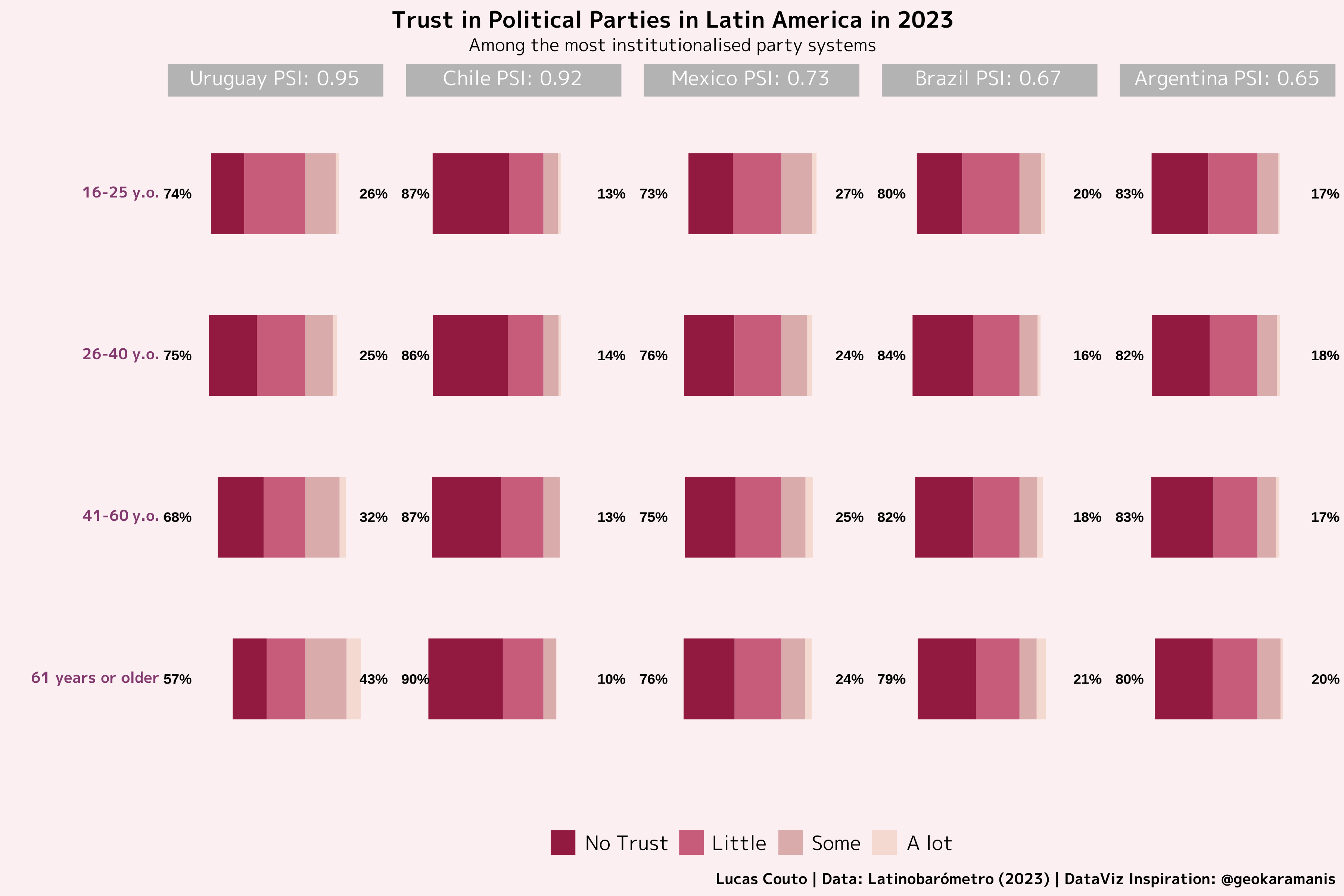
Without further ado, this month my inspiration comes from @geokaramanis. With mass public data from Latinobarómetro, I examine to what extent trust in parties varies according to different group ages. Filtering the data to analyse only the countries with the most institutionalised party systems in 2023,¹ the picture is quite gloomy. Except for the most senior group age from Uruguay, every group age nourishes a profound distrust of parties among the countries with most institutionalised party systems. To say the least, this is very worrying.

See you next month!

Trust in Parties in Latin America across different cohorts

Code

Show the code

##before you proceed, you should download the data from https://www.latinobarometro.org/latContents.jsp

#Packages
library(ggtext)
library(ggstats)
library(haven)
library(ragg)
library(readxl)
library(showtext)
library(tidyverse)

#functions to be used
`%notin%` <- Negate(`%in%`)


#Data Wrangling
latin <- read_dta("Latinobarometro_2023_Eng_Stata_v1_0.dta")

age_levels <- c("16-25 y.o.",
                "26-40 y.o.",
                "41-60 y.o.",
                "61 years or older")

trust_levels <- c("No Trust",
                  "Little",
                  "Some",
                  "A lot")

latin1 <- latin %>% 
          mutate(age_category = case_when(reedad == 1 ~ "16-25 y.o.",
                                          reedad == 2 ~ "26-40 y.o.",
                                          reedad == 3 ~ "41-60 y.o.",
                                          reedad == 4 ~ "61 years or older",
                                          reedad < 0 ~ "DNK / DNA")) %>% 
          filter(idenpa > 1) %>%
          filter(idenpa %in% c(32, 76, 152, 484, 858)) %>%
          mutate(country = case_when(idenpa == 32 ~ "Argentina\n PSI: 0.65",
                                     idenpa == 76 ~ "Brazil\n PSI: 0.67",
                                     idenpa == 152 ~ "Chile\n PSI: 0.92",
                                     idenpa == 484 ~ "Mexico\n PSI: 0.73",
                                     idenpa == 858 ~ "Uruguay\n PSI: 0.95")) %>%
          mutate(country = fct_relevel(country, "Uruguay\n PSI: 0.95", "Chile\n PSI: 0.92", 
                                                "Mexico\n PSI: 0.73", "Brazil\n PSI: 0.67",
                                                "Argentina\n PSI: 0.65")) %>%
          filter(P13ST_G > 0) %>%
          mutate(trust_party = case_when(P13ST_G == 1 ~ "A lot",
                                         P13ST_G == 2 ~ "Some",
                                         P13ST_G == 3 ~ "Little",
                                         P13ST_G == 4 ~ "No Trust",
                                         P13ST_G < 0 ~ "DNK / DNA")) %>%
          mutate(age_category = fct_relevel(age_category, age_levels),
                 trust_party = fct_relevel(trust_party, trust_levels)) %>% 
          count(age_category, country, trust_party)

#fonts
font_add(family = "regular", "MPLUS1p-Regular.ttf")
font_add(family = "bold", "MPLUS1p-Bold.ttf")
showtext_auto() 

#plot
plot <- gglikert(latin1, trust_party, y = age_category, weight = n,
         facet_cols = vars(country), facet_label_wrap = 34, totals_include_center = T,
         add_labels = FALSE, totals_fontface = "bold",
         labels_size = 10, width = 0.5) +
        scale_fill_manual(values = c("#921A40", "#C75B7A", "#D9ABAB","#F4D9D0")) + 
        coord_cartesian(clip = "off") +
        guides(fill = guide_legend(nrow = 1)) +
        labs(title = "Trust in Political Parties in Latin America in 2023",
             subtitle = "Among the most institutionalised party systems",
             x = "", y = "",
            caption = "Lucas Couto | Data: Latinobarómetro (2023) | DataViz Inspiration: @geokaramanis") +
        theme(
           #Title, Subtitle, Caption
           plot.title = element_text(family = "bold", hjust = 0.5, vjust = 0.5, size = 45, color = "black"),
           plot.title.position = "plot",
           plot.subtitle = element_text(family="regular", size = 35, hjust = 0.5, color = "black"),
           plot.caption = element_text(family="bold", size = 30, color = "black", hjust = 1),
           plot.caption.position = "plot",
           #Panel and Background
           panel.border = element_blank(),
           panel.grid.major = element_blank(),
           panel.grid.minor = element_blank(),
           panel.background = element_rect(fill = "#FBEFF2"),
           plot.background = element_rect(fill = "#FBEFF2", linetype = 'blank'),
           #Axes
           axis.title = element_text(size = 40, family = "regular", color = "#833A6F"),
           axis.text.y = element_markdown(size = 30, family = "bold", color = "#833A6F"),
           axis.text.x = element_blank(),
           axis.ticks = element_blank(),
           axis.line = element_blank(),
           #Plus
           text = element_text(family = "regular", size = 50),
           legend.position = "bottom",
           legend.background = element_rect(fill = "#FBEFF2"),
           panel.spacing.x = unit(1, "line"),
           strip.text = element_markdown())  

#save
ggsave("latin_baro.png",
       plot = plot,
       device = agg_png(width = 12, height = 8, units = "in", res = 300))

Footnotes

These data are sourced from Varieties of Democracy (V-Dem). More specifically, I make use of the vs212 variable↩︎